Box Office Revenue Predictor
Summary
Hollywood Blockbuster is a movie box-office revenue prediction. In this project, we consider this as a multiclassification problem, where the movie revenue is discretized into 9 Category ranging from lowest 1 to highest (a blockbuster) 9. Here, I built and compared the performance of few classifiers: Logistic Regression (LR), Decision Tree Classifier (DTC) and Random Forest Classifier (RFC) to predict revenue categories for a given dataset. The RFC model is shown to perform significantly better than both LR and DTC, with a Bingo Classification Accuracy of 76.6% and a 1-Away Classification Accuracy of 98.0% which is higher than those reported in http://www1.mmo.org.tr/resimler/dosya_ekler/c5b45ddb3ff1f62_ek.pdf
The detailed procedure of building these machine learning (ML) models will be explained in this notebook through the following steps:
- Data Preparation
- EDA
- Feature engineering
- Build & deploy ML model
- Conclusion
Import libraries
import numpy as np # linear algebra
import pandas as pd # data processing
import dill
import matplotlib.pyplot as plt # data visualization
plt.style.use('fivethirtyeight')
import missingno as msno
from collections import Counter, OrderedDict
from wordcloud import WordCloud, STOPWORDS, ImageColorGenerator
import plotly.graph_objs as go
import plotly.offline as py
import warnings
warnings.filterwarnings("ignore")
# nlp- spacy
import re
import spacy
from spacy.lang.en.stop_words import STOP_WORDS
nlp = spacy.load("en_core_web_sm")
#sklearn
from sklearn.feature_extraction.text import TfidfTransformer, TfidfVectorizer, CountVectorizer
from sklearn.linear_model import RidgeCV, LinearRegression, LogisticRegression
from sklearn.svm import SVC
from sklearn.ensemble import RandomForestClassifier
from sklearn.model_selection import GridSearchCV

from sklearn.model_selection import train_test_split
from sklearn.preprocessing import OneHotEncoder, StandardScaler
from sklearn.pipeline import Pipeline
from sklearn.compose import ColumnTransformer

from sklearn.metrics import confusion_matrix, accuracy_score, precision_score, recall_score, f1_score
from sklearn. metrics import classification_report
try:
    import eli5
except ImportError as e:
    ! pip install eli5
    import eli5
1. Data preparation
Two Training and Scoring datasets are provided. In the former that will be used to train our model, other than the target variable Category and its continuum counterpart total, there are 12 features for each movie including: name, production year, production method, genre, language, etc. The latter is our test dataset (unseen data) for which we are supposed to predict movie revenue categories. Data preparation includes:
- Loading data, data cleaning, and data enrichment (if it is required)
- In this particular case I used the provided data and did not add data from an external source. However, in practice, it is always a good idea to gather further data to improve a model.
scoring = pd.read_excel('../../datacourse/hollywoodcasestudyhosseinaziziquantiphiinterview/Scoring Sheet.xlsx')
training = pd.read_excel('../../datacourse/hollywoodcasestudyhosseinaziziquantiphiinterview/Training sheet.xlsx')

# Reading train & test data into DataFrames
df_score = pd.read_excel('../hollywoodcasestudyhosseinaziziquantiphiinterview/Scoring Sheet.xlsx')
df_train = pd.read_excel('../hollywoodcasestudyhosseinaziziquantiphiinterview/Training sheet.xlsx')
# Dataframe info
df_train.info(verbose=True)
<class 'pandas.core.frame.DataFrame'>
RangeIndex: 1196 entries, 0 to 1195
Data columns (total 15 columns):
 #   Column                              Non-Null Count  Dtype
---  ------                              --------------  -----
 0   id                                  1196 non-null   int64
 1   name                                1196 non-null   object
 2   display_name                        1196 non-null   object
 3   production_year                     1196 non-null   int64
 4   movie_sequel                        1196 non-null   int64
 5   creative_type                       1196 non-null   object
 6   source                              1196 non-null   object
 7   production_method                   1196 non-null   object
 8   genre                               1196 non-null   object
 9   language                            1196 non-null   object
 10  board_rating_reason                 1196 non-null   object
 11  movie_board_rating_display_name     1196 non-null   object
 12  movie_release_pattern_display_name  1196 non-null   object
 13  total                               1196 non-null   int64
 14  Category                            1196 non-null   int64
dtypes: int64(5), object(10)
memory usage: 140.3+ KB
df_score.info(verbose=True)
<class 'pandas.core.frame.DataFrame'>
RangeIndex: 91 entries, 0 to 90
Data columns (total 14 columns):
 #   Column                              Non-Null Count  Dtype
---  ------                              --------------  -----
 0   id                                  91 non-null     int64
 1   name                                91 non-null     object
 2   display_name                        91 non-null     object
 3   production_budget                   91 non-null     int64
 4   production_year                     91 non-null     int64
 5   movie_sequel                        91 non-null     int64
 6   creative_type                       91 non-null     object
 7   source                              91 non-null     object
 8   production_method                   91 non-null     object
 9   genre                               91 non-null     object
 10  language                            91 non-null     object
 11  board_rating_reason                 91 non-null     object
 12  movie_board_rating_display_name     91 non-null     object
 13  movie_release_pattern_display_name  91 non-null     object
dtypes: int64(4), object(10)
memory usage: 10.1+ KB
There is no null entiries in niether of training or scoring data
print("Training dataset - number of observations: {}, number of features: {}".format(*df_train.shape))
print("Scoring dataset  - number of observations: {}, number of features: {}".format(*df_score.shape))
Training dataset - number of observations: 1196, number of features: 15
Scoring dataset  - number of observations: 91, number of features: 14
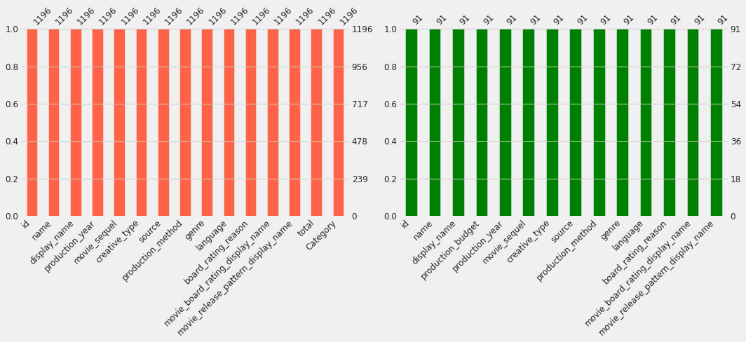
Missing data
One can visualize the presence and distribution of missing data within a pandas dataFrame. It seems that there is no missing data here.
fig = plt.figure(figsize=(15,7))

# traning dataset
ax1 = fig.add_subplot(1,2,1)
msno.bar(df_train, color="tomato", fontsize=12, ax=ax1);

# scoring datset
ax2 = fig.add_subplot(1,2,2)
msno.bar(df_score, color="green", fontsize=12, ax=ax2);

plt.tight_layout()
To confirm that there is no missing data:
df_train.isna().sum()
id                                    0
name                                  0
display_name                          0
production_year                       0
movie_sequel                          0
creative_type                         0
source                                0
production_method                     0
genre                                 0
language                              0
board_rating_reason                   0
movie_board_rating_display_name       0
movie_release_pattern_display_name    0
total                                 0
Category                              0
dtype: int64
df_score.isna().sum()
id                                    0
name                                  0
display_name                          0
production_budget                     0
production_year                       0
movie_sequel                          0
creative_type                         0
source                                0
production_method                     0
genre                                 0
language                              0
board_rating_reason                   0
movie_board_rating_display_name       0
movie_release_pattern_display_name    0
dtype: int64
Duplications
# find all duplications based on all columns of the datasets
print("Number of duplicated rows in the training dataset: {}, and in scoring dataset: {}".\
      format(df_train.duplicated().sum(), df_score.duplicated().sum()))
Number of duplicated rows in the training dataset: 0, and in scoring dataset: 0
Check statistics
df_train.describe()
| id | production_year | movie_sequel | total | Category | |
|---|---|---|---|---|---|
| count | 1.196000e+03 | 1196.000000 | 1196.000000 | 1196.000000 | 1196.000000 |
| mean | 8.928203e+07 | 2008.984950 | 0.097826 | 104.703177 | 3.564381 |
| std | 4.832893e+07 | 1.383625 | 0.297204 | 181.927715 | 1.962417 |
| min | 7.011500e+04 | 2007.000000 | 0.000000 | 1.000000 | 1.000000 |
| 25% | 4.808012e+07 | 2008.000000 | 0.000000 | 11.000000 | 2.000000 |
| 50% | 9.391012e+07 | 2009.000000 | 0.000000 | 40.500000 | 3.000000 |
| 75% | 1.354326e+08 | 2010.000000 | 0.000000 | 114.250000 | 5.000000 |
| max | 1.769701e+08 | 2011.000000 | 1.000000 | 2784.000000 | 9.000000 |
</div>
df_score.describe()
| id | production_budget | production_year | movie_sequel | |
|---|---|---|---|---|
| count | 9.100000e+01 | 9.100000e+01 | 91.0 | 91.000000 |
| mean | 1.607254e+08 | 2.387033e+07 | 2012.0 | 0.208791 |
| std | 2.756827e+07 | 5.614419e+07 | 0.0 | 0.408697 |
| min | 7.970115e+06 | 0.000000e+00 | 2012.0 | 0.000000 |
| 25% | 1.597501e+08 | 0.000000e+00 | 2012.0 | 0.000000 |
| 50% | 1.693001e+08 | 0.000000e+00 | 2012.0 | 0.000000 |
| 75% | 1.719101e+08 | 1.275000e+07 | 2012.0 | 0.000000 |
| max | 1.819001e+08 | 2.700000e+08 | 2012.0 | 1.000000 |
2. Exploratory data analysis (EDA)
- In this stage I used data visualization techniques to see the relation between features and the target variable.
- To better understand and visualize the underlying correlations, I used continuum variable
totalas the target variable.
2.1 Total
This is the feature based on which Category is defined. It cannot be used in our predictive model. However, we still can exploit it to capture the relation of the features to the target label. Throughout this notebook, the word revenue is used interchangeably with total.
# sns.histplot(training.total, kde=True)
fig, ax = plt.subplots(figsize = (14, 4))

plt.subplot(1, 2, 1)
sns.histplot(df_train['total'], kde=True);
plt.xlabel('Distribution of total gross earnings (in Millions of $ ) ');

plt.subplot(1, 2, 2)
# sns.histplot(np.log1p(df_train['total']), kde=True);
sns.histplot(df_train['total'].apply(np.log), bins=20, kde=True);
plt.xlabel('Distribution of log of total gross earnings ');
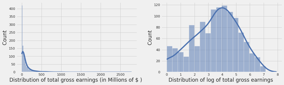
The total distribution is highly skewed. I will use np.log1p(total) instead which is closer to normal distribution.
2.2 Display name
Top words
plt.figure(figsize = (8,8))
text =  df_train.display_name.to_string()
wordcloud = WordCloud(max_font_size=None, background_color='black', width=1200, height=1000).generate(text)
plt.imshow(wordcloud)
plt.title('Top words in movie display name')
plt.axis("off")
plt.show()
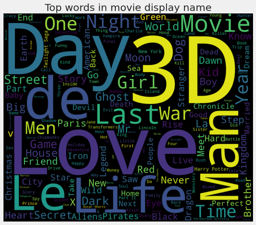
It seems that there are words like 3D or Love that are common in movie names and might be correlated to movie success. This will be inspected during the feature engineering.
2.3 Production year
fig, ax = plt.subplots(1, 2, figsize=(10, 4))
year_counts = df_train.production_year.value_counts().sort_index(ascending=True)
df_year_med_total = df_train.groupby('production_year')['total'].median().sort_index()
sns.barplot(x=year_counts.index, y=year_counts.values, ax=ax[0])
sns.barplot(x=df_year_med_total.index, y=df_year_med_total.values, ax=ax[1])

ax[0].set_title('Count movies per year', size=10)
ax[1].set_title('Median revenue by year (milions $)', size=10)
ax[0].set_xlabel('Year')
ax[1].set_xlabel('Year')
plt.tight_layout()
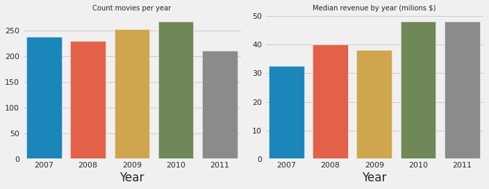
The total-year plot seems to indicate revenue has been increasing over the years. It should be noted that this might be related to the increase of ticket price.
2.4 Movie sequel
fig, ax = plt.subplots(1, 2, figsize=(12, 4))
df_train.movie_sequel.value_counts().plot.bar(ax=ax[0])
sns.boxplot(x='movie_sequel', y=np.log1p(df_train['total']), data=df_train, ax=ax[1])
ax[0].set_title("Count by movie sequel", size=10)
ax[1].set_ylabel('Log total', fontsize=10)
ax[1].set_title("Log revenue by movie sequel (Millions of $)", size=10)
ax[1].set_xlabel("")
plt.tight_layout()
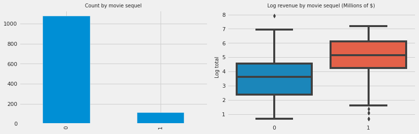
Although the number of movies with sequel is much less than those without sequel, the former seems to have a positive effect on the total gross income.
2.5 Creative type
fig, ax = plt.subplots(1, 2, figsize=(15,7))
df_train.creative_type.value_counts().plot.barh(ax=ax[0]);
df_train.groupby('creative_type')['total'].median().sort_values(ascending=False).plot.barh(ax=ax[1])
ax[0].set_title("Count by creative type", size=15)
ax[1].set_title("Meadian total by creative type  (milions $)", size=15)
ax[1].set_ylabel("Creative type")
plt.tight_layout()
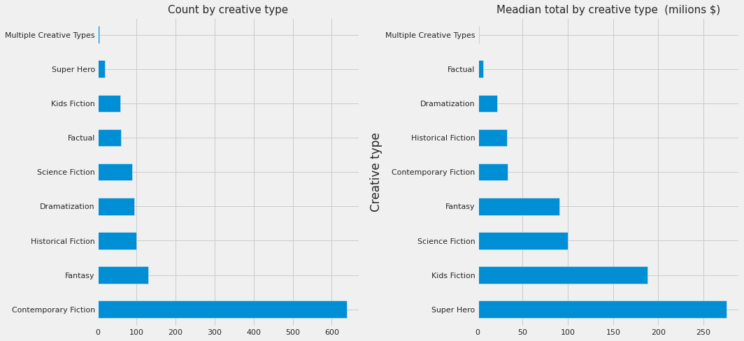
Different creative type seems to have an effect on the revenue.
2.6 Source
fig, ax = plt.subplots(1, 2, figsize=(15,7))
df_train.source.value_counts().plot.barh(ax=ax[0]);
df_train.groupby('source')['total'].median().sort_values(ascending=False).plot.barh(ax=ax[1])
ax[0].set_title("Count by source", size=15)
ax[1].set_title("Meadian total by source  (milions $)", size=15)
plt.tight_layout()
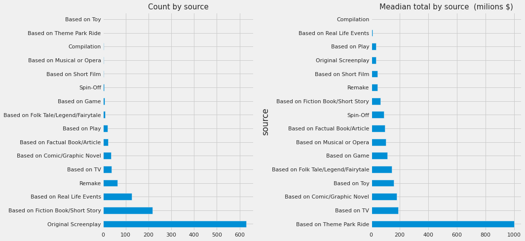
The plots suggest that the movies with certain sources tend to have higher revenues. However, there are few cases where the revenue is very high for the sources with very low counts. For e.g. Based on Theme Park Ride. Let’s take a look at these cases:
df_train.groupby('source')['total'].median().sort_values(ascending=False)
source
Based on Theme Park Ride               1002.5
Based on TV                             189.5
Based on Comic/Graphic Novel            180.0
Based on Toy                            160.0
Based on Folk Tale/Legend/Fairytale     145.5
Based on Game                           116.0
Based on Musical or Opera               103.5
Based on Factual Book/Article            96.0
Spin-Off                                 92.0
Based on Fiction Book/Short Story        66.5
Remake                                   47.0
Based on Short Film                      44.0
Original Screenplay                      35.0
Based on Play                            34.0
Based on Real Life Events                12.0
Compilation                               1.0
Name: total, dtype: float64
df_train.source.value_counts()
Original Screenplay                    629
Based on Fiction Book/Short Story      218
Based on Real Life Events              128
Remake                                  65
Based on TV                             38
Based on Comic/Graphic Novel            36
Based on Factual Book/Article           23
Based on Play                           21
Based on Folk Tale/Legend/Fairytale     10
Based on Game                            8
Spin-Off                                 5
Based on Short Film                      4
Based on Musical or Opera                4
Compilation                              3
Based on Theme Park Ride                 2
Based on Toy                             2
Name: source, dtype: int64
for instance for Based on Theme Park Ride
df_train[df_train.source == 'Based on Theme Park Ride']
| id | name | display_name | production_year | movie_sequel | creative_type | source | production_method | genre | language | board_rating_reason | movie_board_rating_display_name | movie_release_pattern_display_name | total | Category | |
|---|---|---|---|---|---|---|---|---|---|---|---|---|---|---|---|
| 4 | 91700115 | Pirates of the Caribbean 4 | Pirates of the Caribbean: On Stranger Tides | 2011 | 1 | Fantasy | Based on Theme Park Ride | Live Action | Adventure | English | for intense sequences of action/adventure viol... | PG-13 | Wide | 1044 | 9 |
| 7 | 91710115 | Pirates of the Caribbean: At Worlds End | Pirates of the Caribbean: At World's End | 2007 | 1 | Historical Fiction | Based on Theme Park Ride | Live Action | Adventure | English | for intense sequences of action/adventure viol... | PG-13 | Wide | 961 | 9 |
By looking at the data for this particular case, one can see that there are only two movies with this specific source, which may lead to over- or underestimations of revenue due to small sample size. However, we should note that source feature, although it is important, its contribution may not be as significant as other predictors in our model. In other words, there are other features in these observations which can improve our label predictions. Therefore, we do not remove these observations. Besides, it’s better to have a noisy but large dataset than a clean and small one.
2.7 Production method
fig, ax = plt.subplots(2, 1, figsize=(15,7))
df_train.production_method.value_counts().plot.barh(ax=ax[0]);
df_train.groupby('production_method')['total'].median().sort_values(ascending=False).plot.barh(ax=ax[1])
ax[0].set_title("Production method by count", size=12)
ax[1].set_title("Meadian total by production method (milions $)", size=12)
ax[1].set_ylabel("")
plt.tight_layout()
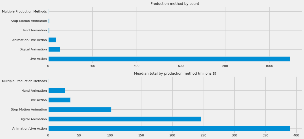
From these plots, one can see that different production methods seem to be making different revenues. Animation/Live Action has the highest and Multiple Production Method has the lowest median total gross revenue.
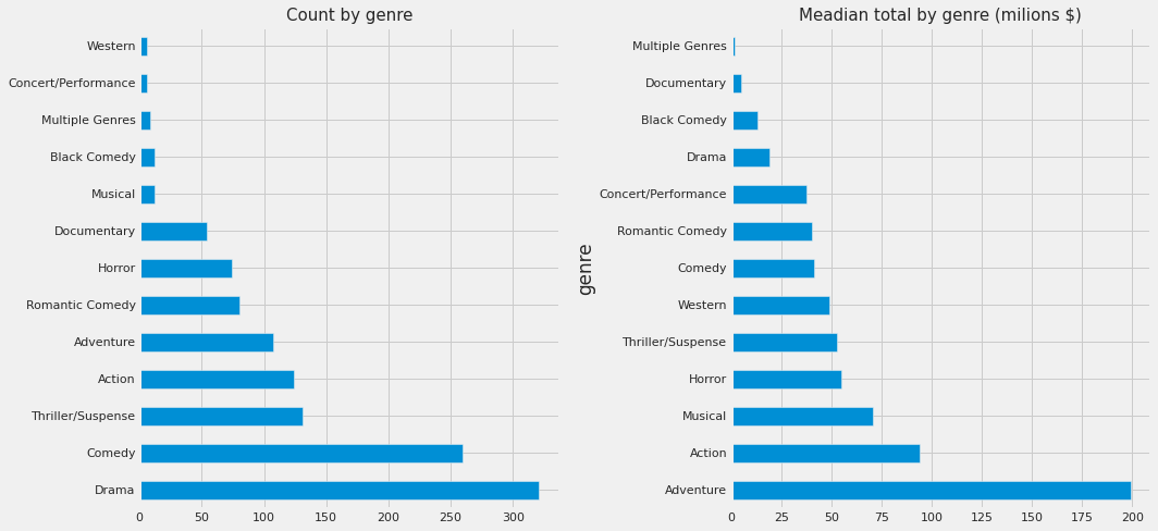
2.8 Genre
fig, ax = plt.subplots(1, 2, figsize=(15,7))
df_train.genre.value_counts().plot.barh(ax=ax[0]);
df_train.groupby('genre')['total'].median().sort_values(ascending=False).plot.barh(ax=ax[1])
ax[0].set_title("Count by genre", size=15)
ax[1].set_title("Meadian total by genre (milions $)", size=15)
plt.tight_layout()
2.9 Language
fig, ax = plt.subplots(1, 2, figsize=(15, 7))
df_train.language.value_counts().sort_values(ascending=False).plot.bar(ax=ax[0])
sns.boxplot(df_train.language, y=np.log1p(df_train['total']), ax=ax[1])
plt.xticks(rotation=90);
plt.tight_layout()
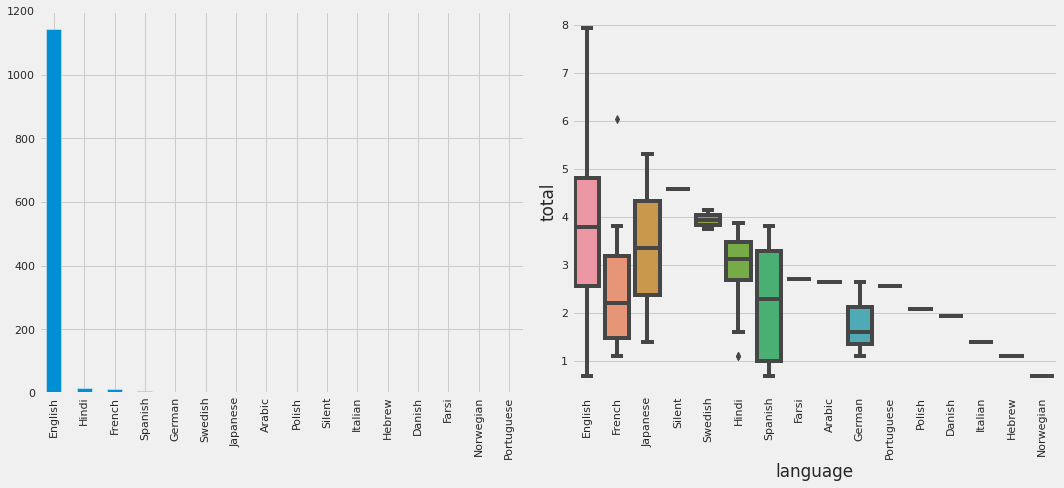
lang_counts = df_train.groupby('language').id.count().sort_values(ascending=False)
Although the majority of the movies are in English, this feature might still improve the accuracy of our movie box office success, particularly when it comes to non-English movies.
2.10 movie_board_rating_display_name
fig, ax = plt.subplots(2, 1, figsize=(15,7))
X = df_train.movie_board_rating_display_name.value_counts().sort_values(ascending=False)
Y = df_train.groupby('movie_board_rating_display_name')['total'].median().sort_values(ascending=False)
sns.barplot(X.values, X.index, ax=ax[0])
sns.barplot(Y.values, Y.index, ax=ax[1])
ax[0].set_title("Rating by count", size=15)
ax[0].set_ylabel("Rating")
ax[1].set_title("Median revenue by rating (milions $)", size=15)
ax[1].set_ylabel("Rating");
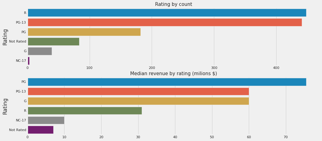
And we can see that different Ratings can make difference in total gross revenue.
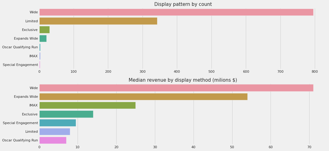
2.11 movie_release_pattern_display_name
fig, ax = plt.subplots(2, 1, figsize=(15,7))

X = df_train.movie_release_pattern_display_name.value_counts().sort_values(ascending=False)
Y = df_train.groupby('movie_release_pattern_display_name')['total'].median().sort_values(ascending=False)

sns.barplot(X.values, X.index, ax=ax[0])
sns.barplot(Y.values, Y.index, ax=ax[1])
ax[0].set_title("Display pattern by count", size=15)
ax[1].set_title("Median revenue by display method (milions $)", size=15)
ax[1].set_ylabel("")
plt.tight_layout()
3. Feature engineering
-
Create numerical features based on the categorical variables (e.g., genre). These features can also be encoded using
One Hot Encoding -
Create new features from text-based features:
- I used NLP techniques along with
bag-of-wordsmodel to explore the impact ofdisplay_name, orboard_rating_reasonon the total gross revenue - Extract number of words and length of text
- I used NLP techniques along with
3.1 Target
As shown in EDA, log(total) distribution has lower skewness compared to total and is a better feature. However, it should be noted that this is for the purpose of feature engineering and both total and log_total columns should be dropped in our model dataset.
# for the "Training"
df_train['log_total'] = df_train['total'].transform(func = lambda x : np.log1p(x))
3.2 Name
Cleaning up the names:
def cleanup_name(text):
    tags = ['the', 'la']
    l = re.split(', | ', str(text))
    if l[-1].strip().lower() in tags:
        return l[-1].strip() + ' ' + ' '.join(x.strip() for x in l[:-1])
    return str(text)
df_train['name'] = df_train['name'].apply(cleanup_name)
3.2.1 Number of words, and length of name
df_train['name_words']  = df_train['name'].astype('str').apply(lambda x: len(x.split(' ')))
df_train["name_length"] = df_train['name'].astype('str').apply(lambda l: len(l))
fig, ax = plt.subplots(figsize=(17, 6))

# Number of words
col11 = df_train.name_words.value_counts().sort_index(ascending=True)
col12 = df_train.groupby('name_words')['log_total'].median().sort_index()


#Length of name
col21 = df_train.name_length.value_counts().sort_index()
col22 = df_train.groupby('name_length')['log_total'].median().sort_index()

plt.subplot(2, 2, 1)
sns.barplot(x=col11.index, y=col11.values)
plt.title("Count by number of words in name", size=15)
plt.xlabel("Number of words", fontsize=10)

plt.subplot(2,2,2)
sns.barplot(x=col12.index, y=col12.values)
plt.xlabel("Number of words",  fontsize=10)
plt.title("Median log-total by number of words (milions $)", size=15)

# plot only first 30 indices
plt.subplot(2,2,3)
sns.barplot(col21[:60].index, col21[:60].values)
plt.xlabel("Length of name",  fontsize=10)
plt.xticks(rotation=90)

plt.subplot(2,2,4)
sns.barplot(col22[:60].index, col22[:60].values)
plt.xlabel("Length of name",  fontsize=10)
plt.xticks(rotation=90)
plt.tight_layout()
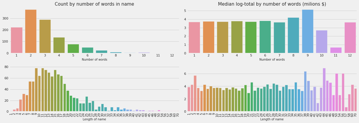
df_train[df_train.name_words == 9]
| id | name | display_name | production_year | movie_sequel | creative_type | source | production_method | genre | language | board_rating_reason | movie_board_rating_display_name | movie_release_pattern_display_name | total | Category | log_total | name_words | name_length | |
|---|---|---|---|---|---|---|---|---|---|---|---|---|---|---|---|---|---|---|
| 16 | 58390115 | Indiana Jones and the Kingdom of the Crystal S... | Indiana Jones and the Kingdom of the Crystal S... | 2008 | 1 | Historical Fiction | Original Screenplay | Live Action | Adventure | English | for adventure violence and scary images. | PG-13 | Wide | 787 | 9 | 6.669498 | 9 | 50 |
| 65 | 83610115 | Night at the Museum 2: Escape from the Smithso... | Night at the Museum: Battle of the Smithsonian | 2009 | 1 | Fantasy | Based on Fiction Book/Short Story | Live Action | Comedy | English | For mild action and brief language | PG | Wide | 413 | 7 | 6.025866 | 9 | 50 |
| 446 | 139860115 | Spy Kids 4 All the Time in the World | Spy Kids: All the Time in the World | 2011 | 1 | Kids Fiction | Original Screenplay | Live Action | Adventure | English | for mild action and rude humor. | PG | Wide | 68 | 4 | 4.234107 | 9 | 36 |
| 952 | 166560115 | Seeking a Friend for the End of the World | Seeking a Friend for the End of the World | 2011 | 0 | Science Fiction | Original Screenplay | Live Action | Comedy | English | for language including sexual references, some... | R | Wide | 8 | 2 | 2.197225 | 9 | 41 |
sns.pairplot(data=df_train, x_vars=['name_words', 'name_length',
                                    'log_total'], y_vars=['name_words','name_length','log_total'], corner=True);
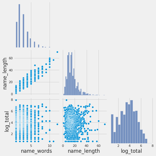
# df_train['log_total'].corr(df_train['name_words'], method='pearson')
df_train['log_total'].corr(df_train['name_length'], method='pearson')
0.026264492327029123
Create similar features for the scoring data:
df_score['name_words']  = df_score['name'].astype('str').apply(lambda x: len(x.split(' ')))
df_score["name_length"] = df_score['name'].astype('str').apply(lambda l: len(l))
3.3 Display_name
3.3.1 Count the number of words in display name
We start by investigating the relation between the content of each movie’s display name and its revenue. We build a linear model predicting the total gross revenue based on the count of the words in each document (bag-of-words model)
def tokenize_lemma(text):
    return [w.lemma_.lower() for w in nlp(text)]

# stop_words_lemma = set(tokenize_lemma(' '.join(STOP_WORDS)))
# stop words
STOP_WORDS = STOP_WORDS.union({'ll', 've', 'pron', 's' , '-pron-'})
stop_words_lemma = set(tokenize_lemma(' '.join(STOP_WORDS)))
# vectorizer = TfidfVectorizer(
#                 sublinear_tf=True,
#                 analyzer='word',
#                 token_pattern=r'\w{1,}', # or alternatively: tokenizer=tokenize_lemma
#                 stop_words=stop_words_lemma,
#                 ngram_range=(1,2) # consider unigram abd bigram
#             )


vectorizer = TfidfVectorizer(
                sublinear_tf=True,
                analyzer='word',
                stop_words=stop_words_lemma,
                ngram_range=(1,2)
        )
y = df_train['log_total']

alphas = [1e-2, 1e-1, 1, 2, 10, 100]

vectorizer.fit(list(df_train['display_name'].astype('str')) + list(df_score['display_name'].astype('str')))
Xtrain_counts = vectorizer.transform(df_train['display_name'].astype('str'))
Xscore_counts = vectorizer.transform(df_score['display_name'].astype('str'))
clf = RidgeCV(alphas=alphas, scoring = 'neg_mean_squared_error',).fit(Xtrain_counts, y)
print("Best alpha paramter: {}, and regression score:{}".format(clf.alpha_, clf.score(Xtrain_counts, y)))
Best alpha paramter: 1.0, and regression score:0.7337945750023136
eli5.show_weights(clf, vec=vectorizer, top=30, feature_filter=lambda x: x != '<BIAS>')
# df_train[df_train.display_name.str.contains('Captain', na=False)]
Create a new feature wcount_dispname based on the prediction of the linear model:
df_train['wpred_dispname'] = clf.predict(Xtrain_counts)
Now let’s take a look at the relation between total and wpred_dispname
sns.jointplot(x="wpred_dispname", y="log_total", data=df_train, kind="reg", line_kws={'color': 'black', "alpha":0.5,"lw":2});
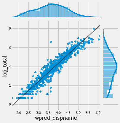
As shown in the figure, there is a linear correlation between prediction of count of words in movie’s name and its revenue. This is a very important feature for our predictive model.
We now use this the fitted model to create a new feature in our df_score dataset.
df_score['wpred_dispname'] = clf.predict(Xscore_counts)
print("score for a display name '{}' in df_score:".format(df_score['display_name'].values[13]))
eli5.show_prediction(clf, doc=df_score['display_name'].values[13], vec=vectorizer)
score for a display name 'Rise of The Guardians' in df_score:
3.3.2 Number of words, and length of display_name
df_train['dispname_words']  = df_train['display_name'].apply(lambda x: len(str(x).split(' ')))
df_train["dispname_length"] = df_train['display_name'].apply(lambda l: len(str(l)))

df_score['dispname_words']  = df_score['display_name'].astype('str').apply(lambda x: len(x.split(' ')))
df_score["dispname_length"] = df_score['display_name'].astype('str').apply(lambda l: len(l))
# find the correlation bwteen features and total
print("Correlation (linear) between '{}' and '{}' is {}".format('log_total', 'dispname_words',
                  df_train['log_total'].corr(df_train['dispname_words'], method='pearson')))

print("Correlation (linear) between '{}' and '{}' is {}".format('log_total', 'dispname_length',
                   df_train['log_total'].corr(df_train['dispname_length'], method='pearson')))
Correlation (linear) between 'log_total' and 'dispname_words' is 0.015313898200359694
Correlation (linear) between 'log_total' and 'dispname_length' is 0.04537696500485102
3.4 Creative type
creativity = df_train.creative_type.unique().tolist()
creativity.extend(df_score.creative_type.unique().tolist())
list_of_creativity = list(set(creativity))
for c in list_of_creativity:
    df_train['cr_' + c] = df_train['creative_type'].apply(lambda x: 1 if c in str(x) else 0)
    df_score['cr_' + c] = df_score['creative_type'].apply(lambda x: 1 if c in str(x) else 0)
3.5 Source
def extract_source(text):
    return ' '.join([str(x).strip() for x in [w for w in nlp(str(text)) if w.tag_ not in ('VBN', 'IN') ]]).replace(' /', ',')
# clean up the source text
df_train['source'] = df_train['source'].apply(extract_source)
df_score['source'] = df_score['source'].apply(extract_source)
list_ = [x.split(',') for x in df_train.source.unique().tolist()]
list_.extend([x.split(',') for x in df_score.source.unique().tolist()])
list_of_source = list(set([x.strip() for item in list_ for x in item]))
Now create features based on the unique sources
for s in list_of_source:
    df_train['source_' + s] = df_train['source'].apply(lambda x: 1 if s in x else 0 )
    df_score['source_' + s] = df_score['source'].apply(lambda x: 1 if s in x else 0 )
3.6 Production method
Create a list of production method
list_ = [x.split('/') for x in df_train.production_method.unique().tolist()]
list_of_prmethod = list(set([x.strip() for item in list_ for x in item]))
Create a feature for each production_methods
for p in list_of_prmethod:
    df_train['pr_' + p] = df_train['production_method'].apply(lambda x: 1 if p in x else 0 )
    df_score['pr_' + p] = df_score['production_method'].apply(lambda x: 1 if p in x else 0 )
3.7 Genre
Create a list of genres
list_of_genres = list(set([item for sublist in [x.split('/') for x in  (df_train.genre.unique().tolist() + \
                                           df_score.genre.unique().tolist()) ] for item in sublist] ))
for g in list_of_genres:
    df_train['gen_' + g] = df_train['genre'].apply(lambda x: 1 if g in x else 0)
    df_score['gen_' + g] = df_score['genre'].apply(lambda x: 1 if g in x else 0)
3.8 Language
We can create features for each language.
langs = df_train.language.unique().tolist() + df_score.language.unique().tolist()
list_of_langs = list(set([item for sublist in [x.split('/') for x in langs] for item in sublist]))
for l in list_of_langs:
    df_train['lang_' + l] = df_train['language'].apply(lambda x: 1 if l in x else 0)
    df_score['lang_' + l] = df_score['language'].apply(lambda x: 1 if l in x else 0)
Another feature is isLanguageEnglish which divides the movies into two English and non-English categories:
df_train['isLanguageEnglish'] = df_train['language'].apply(lambda x: 1 if x == 'English' else 0)
fig, ax = plt.subplots(figsize=(15,4))

plt.subplot(1,2,1)
df_train['isLanguageEnglish'].value_counts().sort_index().plot.bar()
plt.xlabel('isLanguageEnglish', fontsize=12)
plt.ylabel('Counts', fontsize=12)
plt.xticks(rotation=0)

plt.subplot(1,2,2)
sns.boxplot(x='isLanguageEnglish', y='log_total', data=df_train)
plt.xlabel('isLanguageEnglish', fontsize=12)
plt.ylabel('log total (Millions of $)', fontsize=12);
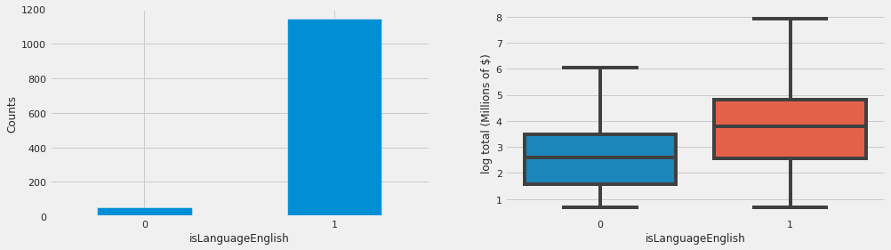
And same feature for the scoring dataset:
df_score['isLanguageEnglish'] = df_score['language'].apply(lambda x: 1 if x == 'English' else 0)
3.9 movie_board_rating_display_name
ratings = df_train.movie_board_rating_display_name.unique().tolist() + df_score.movie_board_rating_display_name.unique().tolist()
list_of_ratings = list(set(ratings))
for r in list_of_ratings:
    df_train['rate_' + r] = df_train['movie_board_rating_display_name'].apply(lambda x: 1 if x == r else 0)
    df_score['rate_' + r] = df_score['movie_board_rating_display_name'].apply(lambda x: 1 if x == r else 0)
3.10 board_rating_reason
This column also contains review text for movie rating, and similar to the display_name, is expected to have significant correlation with total gross revenue and thus with the target label, i.e., Category.
3.10.1 Count the number of words
def clean_rating_text(text_):
#     patt = ['intense sequences', 'sequences', 'intense', 'brief', 'content', 'material', 'strong', 'mild', '-']
    patt = ['-']
    regex = re.compile('|'.join(map(re.escape, patt)))
    tmp = regex.sub("", text_)
    return ', '.join([' '.join([str(w) for w in nlp(x) if w.tag_.startswith(('N', 'J')) ] ) \
                     for x in re.split(' and |, ', tmp.lower(). \
                        replace('/', ' and ').replace(' including ', ' and '))]
                   )
Apply changes to the board_rating_reason column
df_train['new_brr'] = df_train.board_rating_reason.apply(clean_rating_text)
df_score['new_brr'] = df_score.board_rating_reason.apply(clean_rating_text)
vectorizer = TfidfVectorizer(
                sublinear_tf=True,
                analyzer='word',
                token_pattern=r'\w{1,}',
                stop_words=stop_words_lemma,
                ngram_range=(1,2),
                min_df = 2
            )
# X_train_vec = vectorizer.fit_transform(X_train)
Xtrain_brr = df_train['new_brr']
Xscore_brr = df_score['new_brr']
y = df_train['log_total']

vectorizer.fit(list(df_train['new_brr']) + list(df_score['new_brr']))
Xtrain_counts = vectorizer.transform(df_train['new_brr'])
Xscore_counts = vectorizer.transform(df_score['new_brr'])
alphas = [1e-2, 1e-1, 1, 3, 10, 100]
clf = RidgeCV(alphas=alphas, scoring = 'neg_mean_squared_error',).fit(Xtrain_counts, y)
print("Best alpha paramter: {}, and regression score:{}".format(clf.alpha_, clf.score(Xtrain_counts, y)))
Best alpha paramter: 10.0, and regression score:0.3263241905780402
eli5.show_weights(clf, vec=vectorizer, top=20, feature_filter=lambda x: x != '<BIAS>')
Create a new feature based on the linear model:
df_train['wpred_brr'] = clf.predict(Xtrain_counts)
# plt.figure(figsize=(16, 8))
# plt.subplot(1, 2, 1)
# plt.scatter(df_train['bow_brr'], df_train['log_total'])
# plt.title('log of revenue vs. ')
Let’s take a look at the correlations:
sns.jointplot(x="wpred_brr", y="log_total", data=df_train, kind="reg", line_kws={'color': 'black', "alpha":0.5,"lw":2});
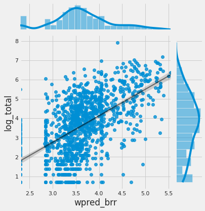
And same for the scoring dataset:
df_score['wpred_brr'] = clf.predict(Xscore_counts)
df_train = df_train.drop(columns='new_brr')
df_score = df_score.drop(columns='new_brr')
1.10.2 Number of words, and length of rating text
df_train['brr_words']  = df_train['board_rating_reason'].apply(lambda x: len(str(x).split(' ')))
df_train["brr_length"] = df_train['board_rating_reason'].apply(lambda l: len(str(l)))
# sns.pairplot(data=df_train, x_vars=['brr_words', 'brr_length',
#                                     'log_total'], y_vars=['brr_words','brr_length','log_total'], corner=True
#             );
# find the correlation bwteen features and total
# print("Correlation (linear) between '{}' and '{}' is {}".format('log_total', 'brr_words',

# print("Correlation (linear) between '{}' and '{}' is {}".format('log_total', 'brr_length',
#                    df_train['log_total'].corr(df_train['brr_length'], method='pearson')))
df_score['brr_words']  = df_score['board_rating_reason'].astype('str').apply(lambda x: len(x.split(' ')))
df_score["brr_length"] = df_score['board_rating_reason'].astype('str').apply(lambda l: len(l))
3. 11 movie_release_pattern_display_name
Create features for movie_release_pattern_display_name column
# clean up the text
df_train['movie_release_pattern_display_name'] = df_train.movie_release_pattern_display_name.apply(lambda x: x.lower())
df_score['movie_release_pattern_display_name'] = df_score.movie_release_pattern_display_name.apply(lambda x: x.lower())
patterns = df_train.movie_release_pattern_display_name.unique().tolist() + \
        df_score.movie_release_pattern_display_name.unique().tolist()
list_of_patterns = list(set(patterns))
for p in list_of_patterns:
    df_train['patt_' + p] = df_train.movie_release_pattern_display_name.apply(lambda x: 1 if x == p else 0)
    df_score['patt_' + p] = df_score.movie_release_pattern_display_name.apply(lambda x: 1 if x == p else 0)
4. Machine learning model
In this section we:
- Prepare train and test data
- Build simple Logistic Regression Classifier model
- Build Decision Tree Classifier
- Improve the performance of the previous model by using random forest classifier model - optimized by GridSearchCV
- Check the feature importance
- Measure the accuracy of our model using Bingo and 1-Away accuracy parameters
- Use the optimized model to predict
Categoryfor the Scoring dataset
4.1 train-test data
# modeling dataFrame
df_model = df_train.copy()
df_valid = df_score.copy()
In case we want to encode categorical features using One Hot Encoder – instead of creating new features. The pipeline:
transformer_name = 'ohe_on_all_categorical_features'
transformer = OneHotEncoder(sparse=False)
columns_to_encode = ['creative_type', 'main_source',
                     'production_method', 'genre',
                     'movie_board_rating_display_name',
                     'movie_release_pattern_display_name']

ohe_final = ColumnTransformer([
    (transformer_name, transformer, columns_to_encode)],
    remainder='passthrough')
cols_to_drop = ['id', 'name', 'display_name', 'creative_type', 'source', 'production_method',
                 'genre', 'language', 'board_rating_reason', 'movie_board_rating_display_name',
                 'movie_release_pattern_display_name', 'Category', 'total', 'log_total'
                ]
valid_cols_to_drop = cols_to_drop[:-3] + ['production_budget']


y = df_model['Category']
X = df_model.drop(columns=cols_to_drop)
X_valid = df_valid.drop(columns=valid_cols_to_drop)
from sklearn.model_selection import train_test_split

X_train, X_test, y_train, y_test = train_test_split(X, y, test_size=0.3, random_state=0, stratify=y)

print("Shape of the complete data set:", X.shape)
print("Shape of the train data set:", X_train.shape)
print("Shape of the test data set:", X_test.shape)
Shape of the complete data set: (1196, 93)
Shape of the train data set: (837, 93)
Shape of the test data set: (359, 93)
I build a pipeline and feed it the original data matrix X. This would easily allow us to make predictions for new data that we might obtain by making our transformations repeatable.
4.2 Logistic Regression
# Set regularization rate
reg = 0.1

# pipeline
lr_pipe = Pipeline([
    ('scalar', StandardScaler()),
    ('lr', LogisticRegression(C=1/reg, solver='lbfgs', multi_class='auto', max_iter=10000))
])

lr_pipe.fit(X_train, y_train);
y_pred = lr_pipe.predict(X_test)

print('Predicted labels: ', y_pred[:20])
print('Actual labels   : ' ,y_test[:20].values)

# Classification report
print(classification_report(y_test, y_pred))
Predicted labels:  [2 5 1 2 3 3 4 3 8 5 3 5 3 1 4 2 4 4 7 6]
Actual labels   :  [2 5 1 2 3 3 4 4 9 5 3 6 4 2 3 2 4 4 5 8]
              precision    recall  f1-score   support

           1       0.79      0.84      0.82        50
           2       0.72      0.68      0.70        74
           3       0.65      0.68      0.66        74
           4       0.64      0.60      0.62        62
           5       0.57      0.65      0.60        40
           6       0.37      0.29      0.33        24
           7       0.24      0.22      0.23        18
           8       0.17      0.27      0.21        11
           9       0.50      0.17      0.25         6

    accuracy                           0.61       359
   macro avg       0.52      0.49      0.49       359
weighted avg       0.62      0.61      0.61       359
4.3 Decision Tree Classifier
from sklearn.tree import DecisionTreeClassifier

# Decision tree Paramters
min_tree_splits = range(2,8)
min_tree_leaves = range(2,8)
nmax_features   = range(1, 60)
max_tree_depth  = range(0,20)
crit            = ['gini', 'entropy']

param_grid = {'max_depth': max_tree_depth,
              'min_samples_split': min_tree_splits,
              'min_samples_leaf': min_tree_leaves,
              "criterion": crit,
              "max_features":nmax_features
             }
# number of crossvalidation folds
cv = 10


# normalize the features
features = Pipeline([
    ('scalar', StandardScaler())
])

# GridSearchCV - classifier
gs = GridSearchCV(
                    DecisionTreeClassifier(),
                    param_grid, cv=cv, n_jobs=-1
            )

DT_est = Pipeline([
                ('feature', features),
                ('gs_est', gs)
            ])

# for the model
DT_est.fit(X_train, y_train);
y_pred = DT_est.predict(X_test)
print('*' * 42)
print('Model performance with Decision Tree'.format(estimatores[0], accuracy_score(y_test, y_pred)))

# Overall metrics
print("Overall Accuracy:",accuracy_score(y_test, y_pred))
print("Overall Precision:",precision_score(y_test, y_pred, average='macro'))
print("Overall Recall:",recall_score(y_test, y_pred, average='macro'))
# print('Average AUC:', roc_auc_score(y_test,label_prob, multi_class='ovr'))
print('*' * 42)

rf_est = DT_est.named_steps['gs_est']
print('*' * 42)
rf_est.best_params_
******************************************
Model performance with Decision Tree
Overall Accuracy: 0.724233983286908
Overall Precision: 0.6448393835648738
Overall Recall: 0.6154484885667681
******************************************
******************************************


{'criterion': 'entropy',
 'max_depth': 5,
 'max_features': 59,
 'min_samples_leaf': 7,
 'min_samples_split': 4}
print("Classification report:")
print(classification_report(y_test, y_pred))
Classification report:
              precision    recall  f1-score   support

           1       0.95      0.80      0.87        50
           2       0.82      0.80      0.81        74
           3       0.74      0.85      0.79        74
           4       0.71      0.76      0.73        62
           5       0.71      0.60      0.65        40
           6       0.71      0.50      0.59        24
           7       0.33      0.44      0.38        18
           8       0.33      0.45      0.38        11
           9       0.50      0.33      0.40         6

    accuracy                           0.72       359
   macro avg       0.64      0.62      0.62       359
weighted avg       0.74      0.72      0.73       359
4.4 Random Forest Classifier
The predicted value of a random forest is just the average of the probabilities of individual trees. To select the best hyperparameters to train the estimator I used GridSearchCV – which is an estimator itself that runs n-fold cross validation on each set of hyperparameters.
# Random Forest Paramters
min_tree_splits = [2] #range(2,8)
min_tree_leaves = [2] #range(2,8)
nmax_features   = [47]#range(1, 100)
max_tree_depth  = [16] #range(0,20)
estimatores     = [100]
bootstrap       = [True, False]
crit            = ['gini', 'entropy']

param_grid = {'max_depth': max_tree_depth,
              'min_samples_split': min_tree_splits,
              'min_samples_leaf': min_tree_leaves,
              "n_estimators": estimatores,
              "bootstrap": bootstrap,
              "criterion": crit,
              "max_features":nmax_features
             }
# number of crossvalidation folds
cv = 10


# normalize the features
features = Pipeline([
    ('scalar', StandardScaler())
])

# GridSearchCV - classifier
gs = GridSearchCV(
                    RandomForestClassifier(random_state = 42),
                    param_grid, cv=cv, n_jobs=-1
            )

pipe = Pipeline([
                ('feature', features),
                ('gs_est', gs)
            ])

# for the model
pipe.fit(X_train, y_train);
with open('rf_est.dill', 'wb') as f:
    dill.dump(pipe, f, recurse=True)
with open('rf_est.dill', 'rb') as f:
    pipe = dill.load(f)
y_pred = pipe.predict(X_test)
print('*' * 42)
print('Model performance with {} decision-trees'.format(estimatores[0], accuracy_score(y_test, y_pred)))

# Overall metrics
print("Overall Accuracy:",accuracy_score(y_test, y_pred))
print("Overall Precision:",precision_score(y_test, y_pred, average='macro'))
print("Overall Recall:",recall_score(y_test, y_pred, average='macro'))
# print('Average AUC:', roc_auc_score(y_test,label_prob, multi_class='ovr'))
print('*' * 42)
******************************************
Model performance with 100 decision-trees
Overall Accuracy: 0.766016713091922
Overall Precision: 0.7103268523297807
Overall Recall: 0.6778578872127258
******************************************
rf_est = pipe.named_steps['gs_est']
print('*' * 42)
rf_est.best_params_
******************************************


{'bootstrap': True,
 'criterion': 'gini',
 'max_depth': 16,
 'max_features': 47,
 'min_samples_leaf': 2,
 'min_samples_split': 2,
 'n_estimators': 100}
print("Classification report:")
print(classification_report(y_test, y_pred))
Classification report:
              precision    recall  f1-score   support

           1       0.91      0.84      0.87        50
           2       0.83      0.78      0.81        74
           3       0.75      0.86      0.81        74
           4       0.79      0.77      0.78        62
           5       0.71      0.68      0.69        40
           6       0.71      0.71      0.71        24
           7       0.57      0.67      0.62        18
           8       0.45      0.45      0.45        11
           9       0.67      0.33      0.44         6

    accuracy                           0.77       359
   macro avg       0.71      0.68      0.69       359
weighted avg       0.77      0.77      0.77       359
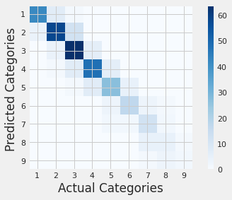
4.5 Confusion matrix
mcm = confusion_matrix(y_test, y_pred)

cats = [str(i+1) for i in range(9) ]

plt.imshow(mcm, interpolation="nearest", cmap=plt.cm.Blues)
plt.colorbar()
tick_marks = np.arange(len(cats))
plt.xticks(tick_marks, cats, rotation=0)
plt.yticks(tick_marks, cats)
plt.xlabel("Actual Categories")
plt.ylabel("Predicted Categories ")
plt.show()
4.6 Feature importance
importances = rf_est.best_estimator_.feature_importances_
feature_names = [f'{i}' for i in X.columns.to_list() ]
fig = plt.subplots(figsize=(15,7))
features = X.columns#df_model.drop(columns=['inventory']).coluns
# importances = best_regress.feature_importances_
# plot top 30 features
indices = np.argsort(importances)[::-1][:30]
# indices = np.argsort(importances)[60:90]
plt.title('Feature Importances')
plt.barh(range(len(indices)), importances[indices], color='b', align='center')
plt.yticks(range(len(indices)), [features[i] for i in indices])
plt.xlabel('Relative Importance')
plt.show()
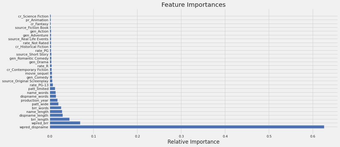
As shown by the feature importance diagram, the word count prediction of movie name (display_name) has the highest impact on the revenue and thus the target labels, followed by word count prediction in board_rating_reason, length of board_rating_reason, display_name, and short name.
4.7 Calculate classification accuracy
def calc_classAccuracy(y_p, y_t):
    ypred = y_p.tolist()
    ytest = y_t.tolist()
    sum_1 = 0
    sum_2 = 0
    for index, label in enumerate(ypred):
        if label == ytest[index]:
            sum_1 += 1
        elif  label == (ytest[index] + 1) or label == (ytest[index] - 1 ):
            sum_2 += 1

    bingo = sum_1/len(ypred)
    One_Away = (sum_1 + sum_2)/len(ypred)
    return print("bingo : {},\n1-Away : {}".format(bingo, One_Away))
calc_classAccuracy(y_pred, y_test)
bingo : 0.766016713091922,
1-Away : 0.9805013927576601
4.8 Unbalance classes
df_train.groupby('Category').id.count().plot.bar();
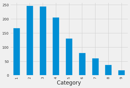
This figure suggests the data set is unbalanced. This might explain the high accuracy over the majority classes, and low accuracy for minority classes. Techniques to deal with unbalanced classes:
- Collect more samples of the minority class in order to have a better representation of it
- undersampling or oversampling each class
- Creating synthetic samples from the minority class can also be effective (e.g., SMOTE)
4.9 Model limitations
-
Lack of conventional variables like budget, historical data for movie release, cast, production company, may hinder the capability for reliable predictions
-
Based on the classification report and confusion matrix the accuracy of some classes are higher than others which can be explained by unbalanced classes
-
The results of this model are only based on 5-year period of data. More data is required for better predictions
-
NLP analysis of text-based features should be performed over longer period of time
4.10 Conclusion
-
The Random Forest model is shown to perform significantly better than a liner model (Logistic Regression) - with a Bingo Classification Accuracy of 76.6% and a 1-Away Classification Accuracy of 98.0%
-
Among the many features that used, the text features are the primary factor to estimate movie box office success
Updates
A.1 Dealing with Imbalanced classes
Number of classes in these observations:
pd.DataFrame((round(df_train['Category'].value_counts().sort_index()/len(df_train), 2)),
    ).reset_index().rename(columns={'index': 'Category', 'Category': 'Value'})
| Category | Value | |
|---|---|---|
| 0 | 1 | 0.14 |
| 1 | 2 | 0.21 |
| 2 | 3 | 0.20 |
| 3 | 4 | 0.17 |
| 4 | 5 | 0.11 |
| 5 | 6 | 0.07 |
| 6 | 7 | 0.05 |
| 7 | 8 | 0.03 |
| 8 | 9 | 0.02 |
For more information about the methods used in this sections, please visit: https://machinelearningmastery.com/bagging-and-random-forest-for-imbalanced-classification/
A.1.1 Cost-sensitive learning - Bootstrap Class Weighting
This technique is used to change the weight of each class in calculating the “impurity” score at a given split point.
# Random Forest Paramters
min_tree_splits = [2] #range(2,8)
min_tree_leaves = [2] #range(2,8)
nmax_features   = [48]#range(1, 50)
max_tree_depth  = [16] #range(0,20)
estimatores     = [100]
bootstrap       = [True, False]
crit            = ['gini', 'entropy']


param_grid = {'max_depth': max_tree_depth,
              'min_samples_split': min_tree_splits,
              'min_samples_leaf': min_tree_leaves,
              "n_estimators": estimatores,
              "bootstrap": bootstrap,
              "criterion": crit,
              "max_features":nmax_features
             }
# number of crossvalidation folds
cv = 10

# normalize the features
features = Pipeline([
    ('scalar', StandardScaler())
])

# GridSearchCV - classifier
gs = GridSearchCV(
                    RandomForestClassifier(random_state = 42, class_weight='balanced_subsample'),
                    param_grid, cv=cv, n_jobs=-1
            )

pipe = Pipeline([
                ('feature', features),
                ('gs_est', gs)
            ])

# for the model
pipe.fit(X_train, y_train);
y_pred = pipe.predict(X_test)
print('*' * 42)
print('Model performance with {} decision-trees with "Bootstrap Class Weighting"'.format(estimatores[0], accuracy_score(y_test, y_pred)))

# Overall metrics
print("Overall Accuracy:",accuracy_score(y_test, y_pred))
print("Overall Precision:",precision_score(y_test, y_pred, average='macro'))
print("Overall Recall:",recall_score(y_test, y_pred, average='macro'))
# print('Average AUC:', roc_auc_score(y_test,label_prob, multi_class='ovr'))
print('*' * 42)
******************************************
Model performance with 100 decision-trees with "Bootstrap Class Weighting"
Overall Accuracy: 0.7604456824512534
Overall Precision: 0.6646570274054403
Overall Recall: 0.6516457660006048
******************************************
print("Classification report using Bootstrap Class Weighting:")
print(classification_report(y_test, y_pred))
Classification report using Bootstrap Class Weighting:
              precision    recall  f1-score   support

           1       0.91      0.82      0.86        50
           2       0.82      0.80      0.81        74
           3       0.76      0.85      0.80        74
           4       0.77      0.77      0.77        62
           5       0.73      0.68      0.70        40
           6       0.72      0.75      0.73        24
           7       0.57      0.67      0.62        18
           8       0.36      0.36      0.36        11
           9       0.33      0.17      0.22         6

    accuracy                           0.76       359
   macro avg       0.66      0.65      0.65       359
weighted avg       0.76      0.76      0.76       359
A.1.2 Random Forest with data undersampling
In this method, the change in the class distribution is done by random under sampling of the majority class.
# random forest with random undersampling for imbalanced classification
from imblearn.ensemble import BalancedRandomForestClassifier
# Random Forest Paramters
min_tree_splits = [2] #range(2,8)
min_tree_leaves = [2] #range(2,8)
nmax_features   = [48]#range(1, 100)
max_tree_depth  = [16]#range(0,20)
estimatores     = [100]
bootstrap       = [True, False]
crit            = ['gini', 'entropy']

param_grid = {'max_depth': max_tree_depth,
              'min_samples_split': min_tree_splits,
              'min_samples_leaf': min_tree_leaves,
              "n_estimators": estimatores,
              "bootstrap": bootstrap,
              "criterion": crit,
              "max_features":nmax_features
             }
# number of crossvalidation folds
cv = 10

# normalize the features
features = Pipeline([
    ('scalar', StandardScaler())
])

# GridSearchCV - classifier
gs = GridSearchCV(
                    BalancedRandomForestClassifier(random_state=42),
                    param_grid, cv=cv, n_jobs=-1
            )

pipe = Pipeline([
                ('feature', features),
                ('gs_est', gs)
            ])

# for the model
pipe.fit(X_train, y_train);
y_pred = pipe.predict(X_test)
print('*' * 42)
print('Model performance with {} decision-trees with data undersampling:'.format(estimatores[0], accuracy_score(y_test, y_pred)))

# Overall metrics
print("Overall Accuracy:",accuracy_score(y_test, y_pred))
print("Overall Precision:",precision_score(y_test, y_pred, average='macro'))
print("Overall Recall:",recall_score(y_test, y_pred, average='macro'))
# print('Average AUC:', roc_auc_score(y_test,label_prob, multi_class='ovr'))
print('*' * 42)
******************************************
Model performance with 100 decision-trees with data undersampling:
Overall Accuracy: 0.754874651810585
Overall Precision: 0.6647875270735196
Overall Recall: 0.6765520750466988
******************************************
print(classification_report(y_test, y_pred))
              precision    recall  f1-score   support

           1       0.82      0.92      0.87        50
           2       0.86      0.77      0.81        74
           3       0.81      0.80      0.80        74
           4       0.75      0.81      0.78        62
           5       0.71      0.68      0.69        40
           6       0.68      0.62      0.65        24
           7       0.48      0.56      0.51        18
           8       0.38      0.27      0.32        11
           9       0.50      0.67      0.57         6

    accuracy                           0.75       359
   macro avg       0.66      0.68      0.67       359
weighted avg       0.76      0.75      0.75       359
pd.DataFrame(confusion_matrix(y_test, y_pred),
            index=[str(i+1) for i in range(9)],
            columns=[str(i+1) for i in range(9)])
| 1 | 2 | 3 | 4 | 5 | 6 | 7 | 8 | 9 | |
|---|---|---|---|---|---|---|---|---|---|
| 1 | 46 | 3 | 1 | 0 | 0 | 0 | 0 | 0 | 0 |
| 2 | 10 | 57 | 7 | 0 | 0 | 0 | 0 | 0 | 0 |
| 3 | 0 | 5 | 59 | 10 | 0 | 0 | 0 | 0 | 0 |
| 4 | 0 | 1 | 5 | 50 | 6 | 0 | 0 | 0 | 0 |
| 5 | 0 | 0 | 1 | 7 | 27 | 5 | 0 | 0 | 0 |
| 6 | 0 | 0 | 0 | 0 | 3 | 15 | 5 | 1 | 0 |
| 7 | 0 | 0 | 0 | 0 | 2 | 2 | 10 | 3 | 1 |
| 8 | 0 | 0 | 0 | 0 | 0 | 0 | 5 | 3 | 3 |
| 9 | 0 | 0 | 0 | 0 | 0 | 0 | 1 | 1 | 4 |
calc_classAccuracy(y_pred, y_test)
bingo : 0.754874651810585,
1-Away : 0.9777158774373259